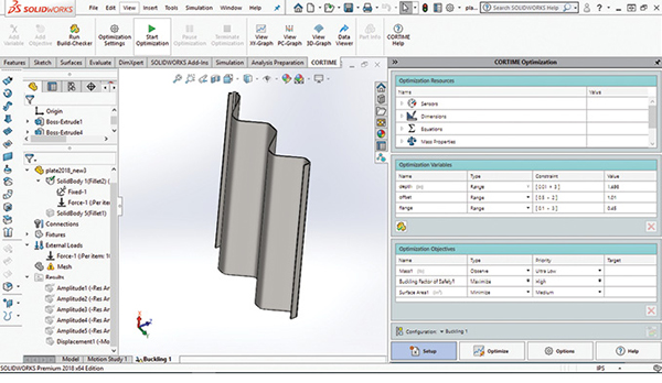
Fig. 3: CORTIME user interface. Images courtesy of Tony Abbey.

Latest News
March 1, 2019
Editor’s Note: Tony Abbey provides live e-Learning courses, FEA consulting and mentoring. Contact tony@fetraining.com for details, or visit his website.
This walkthrough looks at CORTIME, from Apiosoft, a Denmark-based company. CORTIME is a third-party add-in to Dassault Systèmes’ SolidWorks, which provides parametric CAD optimization by driving SolidWorks dimensions and feature controls.
CORTIME uses both SolidWorks geometry responses (known as sensors) such as mass properties, and a range of analysis results (also defined as sensors) from SolidWorks Simulation. This includes all available structural, thermal or computational fluid dynamics (CFD) analyses. CORTIME launched in 2013 and its technology is based on recent research work by the founders.
Parametric Design Optimization
Parametric CAD design optimization assumes the designer has already created some level of formal design within SolidWorks and is on the path to a viable design product. The job of Parametric Design Optimization is to explore varying design parameters and improve the performance of this new design. Changes can be limited to small improvements, effectively polishing the design, or defining configuration in a more generic way, with a wide scope for new and radical configurations to evolve. The accuracy of the responses, such as local stresses, is at the full fidelity of the finite element analysis (FEA) or CFD model.
In my view, parametric design optimization has been somewhat overshadowed by topology optimization. Many designers already have some notion of what structure to put into available design space to carry load, or to support vibration, buckling or whatever the criteria might be. Starting with a blank canvas, such as topology optimization, is not always appropriate.
In this scenario parametric design optimization is a powerful tool. However, the two technologies should not be thought of as competing. Each can produce useful complementary design ideas and information at different stages in the design evolution.
Multi-Objective Optimization
A traditional single objective optimization approach, such as minimizing weight, drives toward an optimum solution, subject to design constraints. For example, an optimum cantilever beam design could seek a minimum weight subject to a limit of tip deflection of 0.1 in. and maximum stress below yield. This represents a single optimum design point.
By contrast, a multi-objective approach could minimize weight, but also attempt to minimize tip deflection. The CORTIME product is built around this multi-objective approach. The motivation for this approach is that most designs are a trade-off.
Sample Study: Panel Buckling
I have been experimenting with CORTIME for several months, exploring how it interacts with SolidWorks Simulation using conventional design variables and feature controls in optimization problems. For this review, I looked at linear buckling, which is a challenging optimization problem as mode shapes and load factors change in a complex way across the design space. I also explored the use of a more generalized geometry forming tool, which is analogous to a manufacturing process. The SolidWorks Deform feature opens up interesting possibilities for generic shape changes. Fig. 1 shows the setup.

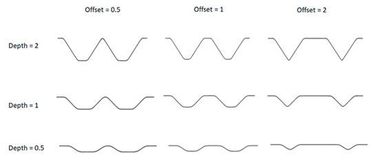
The Deform feature takes the top body, which is the tool and deforms the lower target body, which starts as a flat plate. This gives a form of swaging in the plate. Two design variables are defined in the tool; the depth of the indentors and the offset between them. Together, these give a variety of candidate shapes. A sample of these is shown in Fig. 2.
The Deform feature is interesting, because it attempts to maintain constant volume of material. This means that under the pseudo-forming process, the skins will thin down. This is not an exact forming simulation, but I thought useful as an indication of thickness variation with the stamped design, rather than using a folded sheet design.
The original plate thickness is .05 in. and under the deform action this can reduce to .03 in. or less in the sloped regions. It was important to use the high-fidelity settings, otherwise the geometry will fail in the thin regions. I also meshed the panel using high order Tetrahedral solid elements, so that thickness variation could be represented. The buckling load is sensitive to the local wall thickness, so this was important to include.
Using shell elements is not feasible without complicated mapping to represent the varying thickness. I did a series of benchmarks to compare solid elements vs. shells under buckling for constant thickness and the solid elements performed well.
Setting Up the Problem
Fig. 3 shows the layout of the CORTIME user interface installed as an add-in with the SolidWorks Simulation buckling study setup.
The main interface appears as a task pane on the right-hand side in the figure, with a ribbon above the graphics window. The four tabs at the bottom of the task pane access the initial setup phase, launching and monitoring the optimization phase, additional options and an attractive online help guide.
Most of the functionality can be directly accessed from the ribbon bar, including setting up the optimization, running the optimization and viewing the optimization run using various graphical display methods.
The Setup tab is highlighted in Fig. 3, and the task pane contains forms for accessing the Optimization Resources passed through from SolidWorks, the Optimization Variables defined in CORTIME and the Objective functions defined in CORTIME.
I have defined three sensors in SolidWorks: the Mass, Surface Area of the bottom plate face and the Buckling Factor of Safety. The latter is generated by each SolidWorks Simulation buckling analysis, which is spawned. The Mass is only monitored to check that it stays constant under the Deform feature action. I am using the Surface Area as a gauge of the plate thickness being developed. As the volume is constant, the surface area is an inverse measure of the thickness.
I have used the Equations method to define the depth and offset as global variables within SolidWorks. These are then available to CORTIME. This is slight overkill, as I could have created the dimensions directly as CORTIME variables, on the fly, as they are created. CORTIME appends icons to the menu actions within SolidWorks to set dimensions or feature parameters to be variables or objectives.
I found the global variable approach useful as I could easily replicate a design configuration, using CORTIME variable results on a different installation without CORTIME present. However, to emphasize, as will be seen shortly, working within CORTIME, any design configuration can be easily rebuilt from any of the results graphics windows.
I dragged two global design variables into this window: depth and offset. The Type defines the Range method. The default is to define an upper and lower bound—I like that both values are in one dialog box. Other Range methods include Range with Step, or Range with N-Steps, so you can select specific increments. Range Integer with Step only allows integer values and Discrete Values uses an explicitly defined subset of variables.
I experimented with trial solutions to establish what were sensible ranges. It is a good idea to give the ranges and increments some thought—how do they reflect real-world manufacturing gauges, dimensions and other characteristics? The fewer the number of design variations, the more efficient the optimization run will be. If you are too generous with limits, then resource is wasted exploring the additional design space.
CORTIME has a very useful preview feature called Build-Checker, to help assess ranges. Build-Checker takes the extreme combinations of design variables and creates the corresponding set of geometry configurations automatically. A table of results is presented, indicating successful and failed geometry builds. The failed builds can be clicked on and the geometry failure investigated. As an example, I did a simple plate with a hole stress concentration optimization. The variables were plate width and hole diameter. My variable range allowed the hole to be bigger than the plate width! More complex dimensional interactions are difficult to predict, and Build-Checker does a great job of allowing you to interactively explore and correct design variable ranges.
Back to the objectives created for this optimization study. The Mass is set to Type Observe—I simply want to monitor the value. It should remain constant under the Deform feature operation. The Buckling Factor of Safety is set to Maximize—I want the panel to be resistant to buckling. I have also set the Surface Area to Minimize because I want to reduce the stretching, and hence thinning of the panel.
These are conflicting requirements, so the aim is to produce a set of efficient alternative designs, which satisfy these objectives to a lesser or greater extent. I then make an engineering judgment!
A variation exists on this theme, as I can bias an objective using a Priority level. The default priority levels are set as 3, but you can extend up to 7, which I have done. I set the Factor of Safety to be the dominant objective (high) and the Surface Area as lesser priority (medium). There is a weighting factor of 2 between each level, so in my case the Buckling Factor is twice as important. An equal Priority gives an unbiased search.
Other Objective Types include Target, Avoid Target, Keep Below, Keep Above and Range. Combined with the Priority level, this can give a fascinating range of possibilities. I found them particularly useful when doing a Normal Modes study with frequency band requirements.
It is interesting to note that using Keep Above, or Keep Below, with High or Ultra High Priority is effectively providing a constraint boundary.
The optimization algorithm settings are controlled in the Optimize Task Pane. I selected the default Global Optimization with Initial Randomization. This is recommended by CORTIME as a starting point for a study. The Initial Randomization explores design space, trying to cover the region with a minimum number of exploratory steps. The number of random steps is a function of the Number of Iterations, which CORTIME calculates based on the number of design variables and their ranges. A very good total time estimate can be made by clicking on a calculator icon, which will spawn the current geometry build and its FEA simulation and capture that time.
Other Optimization options include carrying out a fixed Data Sweep, which explores design space in a non-adaptive way. This can be very expensive, but can give insight into what design space looks like. Alternatively, a Response Surface can be generated in an initial session and then used as a surrogate model in a second session. This can be useful in a very expensive analysis such as nonlinear analysis.
Investigating the Results
Users can review various types of result graphs. These are selected at the top of the Optimize task pane, or from the ribbon bar. In Fig. 4 I have used the Progress Graph to check the history of the two design variables.
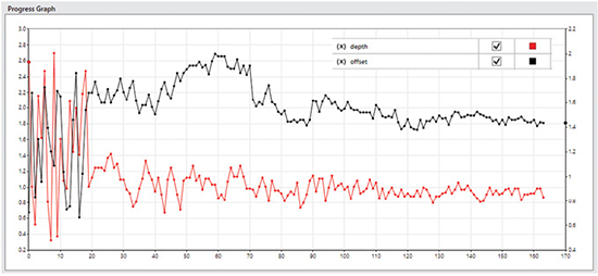
The vertical axes for each variable can be scaled, which is useful for varying orders of the parameter values. Any design variable or objective can be plotted. I have only selected the design variables. The initial random walk can be seen over the first 20 design iterations.
After that, the algorithm takes over and the search tightens up. The fluctuation in variable values can be seen to decay as the steps progress. I have terminated the optimization as the solution focused around one area, but continuing would have reduced the fluctuations further.
For a multi-objective optimization, the solution is not converging to a “best” solution—it is still exploring the trade-off curve. However, in my case, because of the priority given to the Buckling Factor, the results are tending to “bunch” in a particular design space region.
A companion plot is shown in Fig. 5, with the objective function histories shown. The same trend is seen with an initial random walk and then steadily decreasing fluctuations. It is interesting to see that the objective functions show quite significant fluctuations popping up at the final iteration (170), because I have terminated the run before the planned number of iterations—using the “temperature” analogy the system has not fully cooled! In some cases, this would not be wise, if there were likely to be many local optima. In this case, looking at other metrics, I am happy with the data.
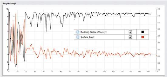
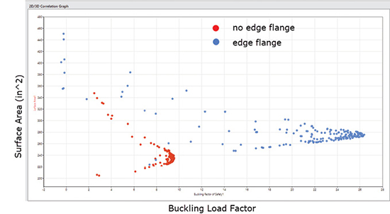
Fig. 6 shows a 2D scatter plot with both objectives plotted in 2D objective space: Surface Area on the vertical axis, Load Factor on the horizontal axis.
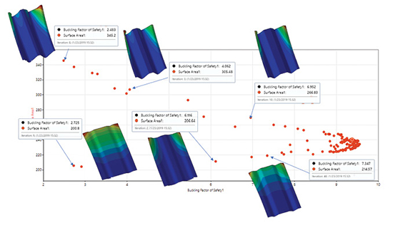
The dots in the scatter plots represent each design and analysis iteration. I have overlaid some representative buckling analysis results. Because of the Buckling Factor emphasis, there are many points clustering towards a high Buckling Factor and corresponding Surface Area region. The “cusp” at the right-hand side of the graph is at a Buckling factor of 9.55 and a surface area of 230 in ^2.
There is a line of results running from this toward the bottom left of the plot. These represent points around the Pareto frontier. I have shown three buckling mode shape results from this line. As a contrast, the upper line of results running from the cusp toward the top left are the most inferior results. They have larger surface areas than designs on the corresponding Pareto curve. I have shown three sample mode shapes from this set.
Between the Pareto frontier (the lower set) and the worse cases (upper set) lie a set of intermediate designs. The strength of the method is that all of these inferior designs can be discarded from trade-off decisions.
The most inferior (upper) set show evidence of local buckling of the deep free edge regions. The lower superior set show varying mode shapes, from some local edge buckling combined with overall buckling (left), local edge buckling (left) and back to combined overall and local buckling (right).
This set can also be thought of as a design trade of curve—low axial loads (Factor 3) can be resisted by a shallow swage with wide offset (left), medium axial loads (Factor 6) can be resisted by a deeper swage with smaller offset and high axial loads (Factor 7.5) can be resisted by a deeper swage and bigger offset.
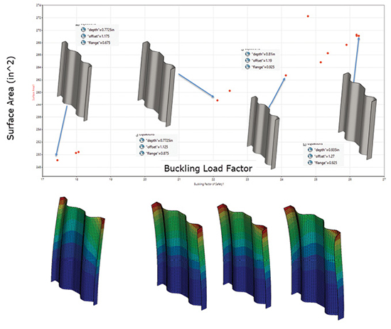
I have ignored the rich set of results around the cusp (Factor 9.5) so far. These are explored in Fig. 7.

Because I biased the Buckling Load Factor over the Surface Area, results have congregated here and allowed a much better Pareto curve definition. I have overlaid the plot with the some of the best candidate designs and their buckling responses. There is a slight tendency toward a non-symmetric free edge buckle at the highest Load Factor, but all designs in this region show a tendency to local edge buckling. There is also a trend toward a deeper and sharper swage to achieve higher Load Factors.
The results can also be filtered to display only the “best” values as defined by CORTIME. These are designs evaluated as best found to date as the algorithm progresses. This filter is shown applied to objectives and variables in Fig. 8.
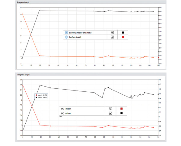
These results are those clustered mainly around the right-hand cusp of Figs. 6 and 7. They show the relative insensitivity of the Load Factor to quite large changes in offset. The depth seems to have stabilized to around 0.75 to 0.8.
Another way to investigate the interaction between design variables and objectives is to plot them all together in a Parallel Coordinate Graph, as shown in Fig. 9.
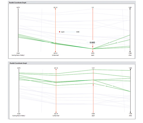
Each of the graph types allows design points to be marked; these points then appear as marked in each of the graphs and highlighted in the Parallel graphs. Fig. 9 contains only the best set, and the vertical axes can be scaled to emphasize the variations. The top graph focuses on the subset of four designs, all with depth of 0.885 in. and shows how they all give very similar objective values. As noted earlier, the result is insensitive to the offset value here.
The bottom graph focuses on the subset of six designs with the highest Load Factor. Most follow the trend that a larger depth and offset gives a higher Load Factor and Surface Area. The steeper the slope between Surface Area and Buckling Factor, the more efficient the design, and this could allow a ranking within this subset.
Redesign Using a Flange
Most of the best designs on the Pareto curve showed local buckling of the free edge, rather than overall buckling. The SolidWorks geometry was modified to include an edge flange of varying height. This kept two objectives but increased the design variables to three.
The results of the second design study are shown superimposed over the original design in Fig. 10. This figure shows the increased effectiveness of the flange, with Load Factors increased up to 26.5. However, as expected, the surface area increases. The mass also jumps to a higher value. A best design curve (Pareto frontier) can be drawn between these two designs.
Finally, Fig. 11 shows the change in buckling mode with the introduction of the edge flanges for the Best set of new designs.
Concluding the Walkthrough
CORTIME provides a well-integrated workflow to carry out Parametric Design Optimization studies across a wide range of analysis types. There’s not enough space to describe all the possibilities in this article, but these include multiple load cases and multi-disciplinary analysis, for example, linking structural, thermal and CFD. I plan to look at non-linear analysis using the surrogate model approach in more detail in a future article.
The results reviewing and interpretation tools allowed for a deeper insight into the exploration of the design and objective space. The ability of the multi-objective approach to evolve design curves or trade-off studies is very powerful.
For More Info
Subscribe to our FREE magazine, FREE email newsletters or both!
Latest News
About the Author
Tony Abbey is a consultant analyst with his own company, FETraining. He also works as training manager for NAFEMS, responsible for developing and implementing training classes, including e-learning classes. Send e-mail about this article to DE-Editors@digitaleng.news.
Follow DE